Spatial autocorrelation

Compute spatial autocorrelation for a numeric vector or a SpatRaster. You can compute standard (global) Moran's I or Geary's C, or local indicators of spatial autocorrelation (Anselin, 1995).

# S4 method for numeric
autocor(x, w, method="moran")

# S4 method for SpatRaster
autocor(x, w=matrix(c(1,1,1,1,0,1,1,1,1),3), method="moran", global=TRUE)

Arguments

x

numeric or SpatRaster

w

Spatial weights defined by or a rectangular matrix. For a SpatRaster this matrix must the sides must have an odd length (3, 5, ...)

global

logical. If TRUE global autocorrelation is computed instead of local autocorrelation

method

character. If x is numeric or SpatRaster: "moran" for Moran's I and "geary" for Geary's C. If x is numeric also: "Gi", "Gi*" (the Getis-Ord statistics), locmor (local Moran's I) and "mean" (local mean)

Value

numeric or SpatRaster

Details

The default setting uses a 3x3 neighborhood to compute "Queen's case" indices. You can use a filter (weights matrix) to do other things, such as "Rook's case", or different lags.

See also

The spdep package for additional and more general approaches for computing spatial autocorrelation

References

Moran, P.A.P., 1950. Notes on continuous stochastic phenomena. Biometrika 37:17-23

Geary, R.C., 1954. The contiguity ratio and statistical mapping. The Incorporated Statistician 5: 115-145

Anselin, L., 1995. Local indicators of spatial association-LISA. Geographical Analysis 27:93-115

https://en.wikipedia.org/wiki/Indicators_of_spatial_association

Examples

### raster
r <- rast(nrows=10, ncols=10, xmin=0)
values(r) <- 1:ncell(r)

autocor(r)
#>    lyr.1 
#> 1.117188 

# rook's case neighbors
f <- matrix(c(0,1,0,1,0,1,0,1,0), nrow=3)
autocor(r, f)
#> lyr.1 
#>  1.25 

# local 
rc <- autocor(r, w=f, global=FALSE)

### numeric (for vector data)
f <- system.file("ex/lux.shp", package="terra")
v <- vect(f)
w <- relate(v, relation="touches")

# global
autocor(v$AREA, w)
#> [1] -0.1531971

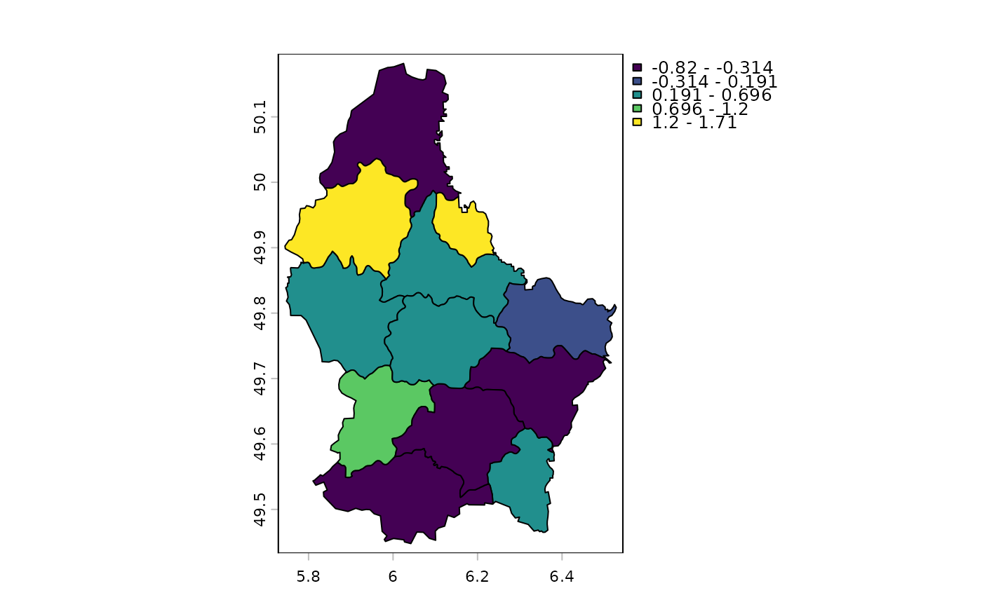
# local
v$Gi <- autocor(v$AREA, w, "Gi") 
plot(v, "Gi")