Make a map

Plot the values of a SpatRaster or SpatVector to make a map.

See points, lines or polys to add a SpatVector to an existing map (or use argument add=TRUE).

There is a separate help file for plotting a SpatGraticule or SpatExtent.

Usage

# S4 method for class 'SpatRaster,numeric'
plot(x, y=1, col, type=NULL, mar=NULL, legend=TRUE, axes=!add, plg=list(), pax=list(), 
    maxcell=500000, smooth=FALSE, range=NULL, fill_range=FALSE, levels=NULL, 
  all_levels=FALSE, breaks=NULL, breakby="eqint", fun=NULL, colNA=NULL, 
  alpha=NULL, sort=FALSE,  reverse=FALSE, grid=FALSE, ext=NULL, reset=FALSE, 
  add=FALSE, buffer=FALSE, background=NULL, box=axes, clip=TRUE, overview=NULL, ...)

# S4 method for class 'SpatRaster,missing'
plot(x, y, main, mar=NULL, nc, nr, maxnl=16, maxcell=500000, add=FALSE, 
  plg=list(), pax=list(), ...)

# S4 method for class 'SpatRaster,character'
plot(x, y, ...)

# S4 method for class 'SpatVector,character'
plot(x, y, col=NULL, type=NULL, mar=NULL, legend=TRUE, axes=!add, plg=list(), pax=list(), 
    main="", grid=FALSE, ext=NULL, sort=TRUE, reverse=FALSE, fun=NULL,
  colNA=NA, alpha=NULL, nr, nc, add=FALSE, buffer=TRUE, background=NULL, 
  box=axes, clip=TRUE, ...)

# S4 method for class 'SpatVector,numeric'
plot(x, y, ...)

# S4 method for class 'SpatVector,missing'
plot(x, y, values=NULL, ...)

# S4 method for class 'SpatVectorCollection,missing'
plot(x, y, main, mar=NULL, nc, nr, maxnl=16, col=NULL, ...)

# S4 method for class 'SpatVectorCollection,numeric'
plot(x, y, main, mar=NULL, ext=NULL, ...)

Arguments

x

SpatRaster or SpatVector

y

missing or positive integer or name indicating the layer(s) to be plotted

col

character vector to specify the colors to use. The default is map.pal("viridis", 100). The default can be changed with the terra.pal option. For example: options(terra.pal=terrain.colors(10)). If x is a SpatRaster, it can also be a data.frame with two columns (value, color) to get a "classes" type legend or with three columns (from, to, color) to get an "interval" type legend. If x us a SpatVectorCollection, a list can be provided with colors for each SpatVector

type

character. Type of map/legend. One of "continuous", "classes", or "interval". If not specified, the type is chosen based on the data

mar

numeric vector of length 4 to set the margins of the plot (to make space for the legend). The default is (3.1, 3.1, 2.1, 7.1) for a single plot with a legend and (3.1, 3.1, 2.1, 2.1) otherwise. The default for a RGB raster is 0. Use mar=NA to not set the margins

legend

logical or character. If not FALSE a legend is drawn. The character value can be used to indicate where the legend is to be drawn. For example "topright" or "bottomleft". Use plg for more refined placement. Not supported for continuous legends (the default for raster data)

axes

logical. Draw axes?

buffer

logical. If TRUE the plotting area is made slightly larger than the extent of x

background

background color. Default is no color (white)

box

logical. Should a box be drawn around the map?

clip

logical. Should the axes be clipped to the extent of x?

overview

logical. Should "overviews" be used for fast rendering? This can result in much faster plotting of raster files that have overviews (e.g. "COG" format) and are accessed over a http connection. However, these overviews generally show aggregate values, thus reducing the range of the actual values. If NULL, the argument is set to TRUE for rasters that are accessed over http and FALSE in other cases

plg

list with parameters for drawing the legend. See the arguments for legend.

A legend can be placed with placed by specifying arguments x and y. For a continuous legend y can have two values. x can also be a SpatExtent. Furthermore, x can have be a keyword such "topleft" and "bottomright" to place the legend at these locations inside the map rectangle. For a continuous legend, only the placement keywords "left", "right", "top", "bottom", "topright", "bottomright" are recognized; and when using these keywords, the legend is placed outside of the map rectangle. The placement of the legend can be altered with argument nudge that move the location in the directions specified with one value (x direction) or two values (x, y). For a continuous legend it can also have four values (xmin, xmax, ymin, ymax). When supplying coordinates, use horiz=TRUE to get a horizontal legend.

Additional parameters for continuous legends include:

digits integer. The number of digits to print after the decimal point
size to change the height and/or width; the defaults are c(1,1)
at to set the location of the tickmarks
format as in formatC to format the numbers. For example, you can use format="g" for scientific notation. The default is "f"
tick One of these partially matched values: "through", "in", "middle", "out", or "none", to choose a tickmark placement/length that is different from the default "throughout".
tick.length to change the tickmark length (default = 1). Only relevant when tick is "throughout" or "out".
tick.col, tick.box.col and tick.lwd to change the appearance of the tickmarks
title.srt to rotate the legend title
title.x and title.y to place the legend title at specific coordinates

pax

list with parameters for drawing axes. See the arguments for axis. Additional parameters include:

side numeric to indicate for which of the axes to draw a line. Default is 1:4 (only noticble when box=FALSE.
tick numeric to indicate for which of the axes to draw tickmarks. Default is 1:2 unless side is changed, in which case the default is the same as side
lab numeric to indicate for which of the axes to draw labels. Default is 1:2 unless side is changed, in which case the default is the same as side
xat/yat numeric with the values at which tickmarks are to be drawn on the horizontal/vertical axis.
xlabs/ylabs this can either be a logical value specifying whether (numerical) annotations are to be made at the tickmarks, or a character or expression vector of labels to be placed at the tickmarks of the horizontal/vertical axis.
retro a logical value that can be set to TRUE to use a sexagesimal notation for the labels (degrees/minutes/hemisphere) instead of the standard decimal notation. For longitude/latitude data only. See graticule for projected data.

maxcell

positive integer. Maximum number of cells to use for the plot

smooth

logical. If TRUE the cell values are smoothed (only if a continuous legend is used)

range

numeric. minimum and maximum values to be used for the continuous legend. You can use NA for one of these to only set the minimum or maximum value

fill_range

logical. If TRUE, values outside of range get the colors of the extreme values; otherwise they get colored as NA

levels

character. labels for the legend when type="classes"

all_levels

logical. If TRUE, the legend shows all levels of a categorical raster, even if they are not present in the data

breaks

numeric. Either a single number to indicate the number of breaks desired, or the actual breaks. When providing this argument, the default legend becomes "interval"

breakby

character or function. Either "eqint" for equal interval breaks, "cases" for equal quantile breaks. If a function is supplied, it should take a single argument (a vector of values) and create groups

fun

function to be called after plotting each SpatRaster layer to add something to each map (such as text, legend, lines). For example, with SpatVector v, you could do fun=function() lines(v). The function may have one argument, representing the layer that is plotted (1 to the number of layers)

colNA

character. color for the NA values

alpha

Either a single numeric between 0 and 1 to set the transparency for all colors (0 is transparent, 1 is opaque) or a SpatRaster with values between 0 and 1 to set the transparency by cell. To set the transparency for a given color, set it to the colors directly

sort

logical. If TRUE legends with categorical values are sorted. If x is a SpatVector you can also supply a vector of the unique values, in the order in which you want them to appear in the legend

reverse

logical. If TRUE, the legend order is reversed

grid

logical. If TRUE grid lines are drawn. Their properties such as type and color can be set with the pax argument

nc

positive integer. Optional. The number of columns to divide the plotting device in (when plotting multiple layers)

nr

positive integer. Optional. The number of rows to divide the plotting device in (when plotting multiple layers)

main

character. Main plot titles (one for each layer to be plotted). You can use arguments cex.main, font.main, col.main to change the appearance; and loc.main to change the location of the main title (either two coordinates, or a character value such as "topleft"). You can also use sub="" for a subtitle. See title

maxnl

positive integer. Maximum number of layers to plot (for a multi-layer object).

add

logical. If TRUE add the object to the current plot

ext

SpatExtent. Can be use instead of xlim and ylim to set the extent of the plot

reset

logical. If TRUE the margins (see argument mar) are reset to what they were before calling plot; doing so may affect the display of additional objects that are added to the map (e.g. with lines)

values

Either a vector with values to be used for plotting or a two-column data.frame, where the first column matches a variable in x and the second column has the values to be plotted

...

arguments passed to plot("SpatRaster", "numeric") and additional graphical arguments

Examples

## SpatRaster
f <- system.file("ex/elev.tif", package="terra") 
r <- rast(f)
plot(r)


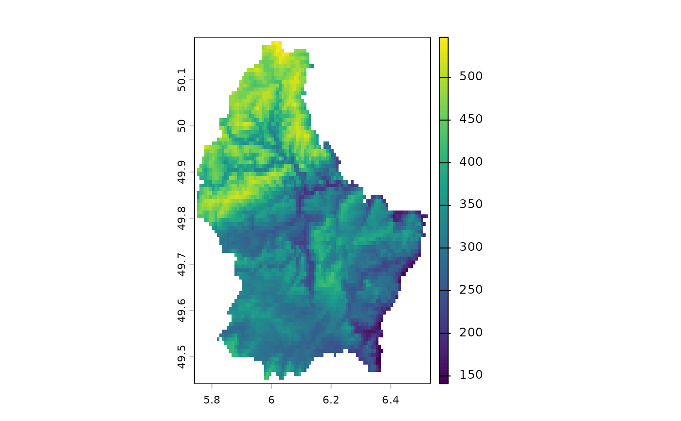plot(r, type="interval")


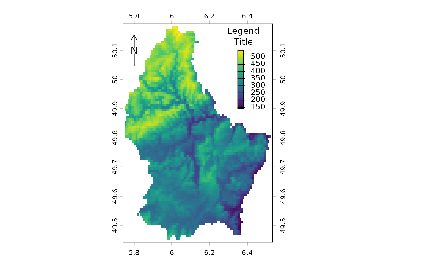
plot(r, plg=list(x=6.35, y = c(49.9, 50.1), title="Legend\nTitle", title.cex=0.9), 
    pax=list(side=1:4, retro=FALSE))
north(cbind(5.8, 50.1))  


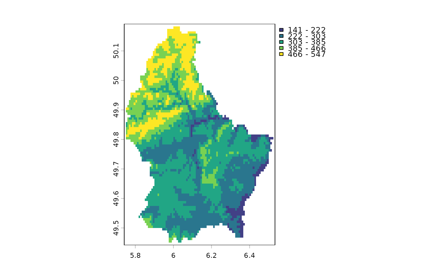
d <- classify(r, c(100,200,300,400,500,600))
plot(d)


plot(d, type="interval", breaks=1:5) 

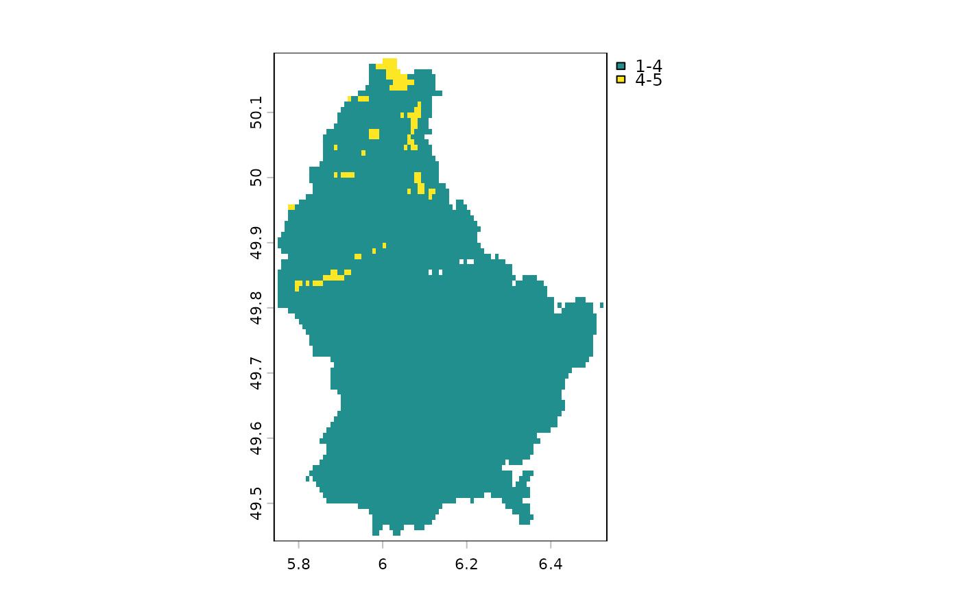
plot(d, type="interval", breaks=c(1,4,5), plg=list(legend=c("1-4", "4-5"))) 

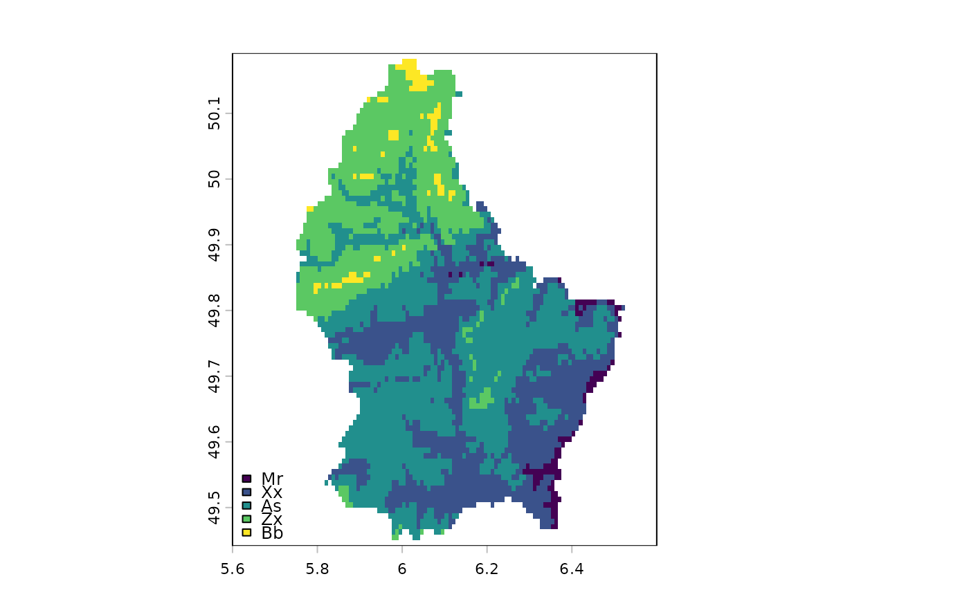
plot(d, type="classes", xlim=c(5.6, 6.6), 
  plg=list(legend=c("Mr", "Xx", "As", "Zx", "Bb"), x="bottomleft"))



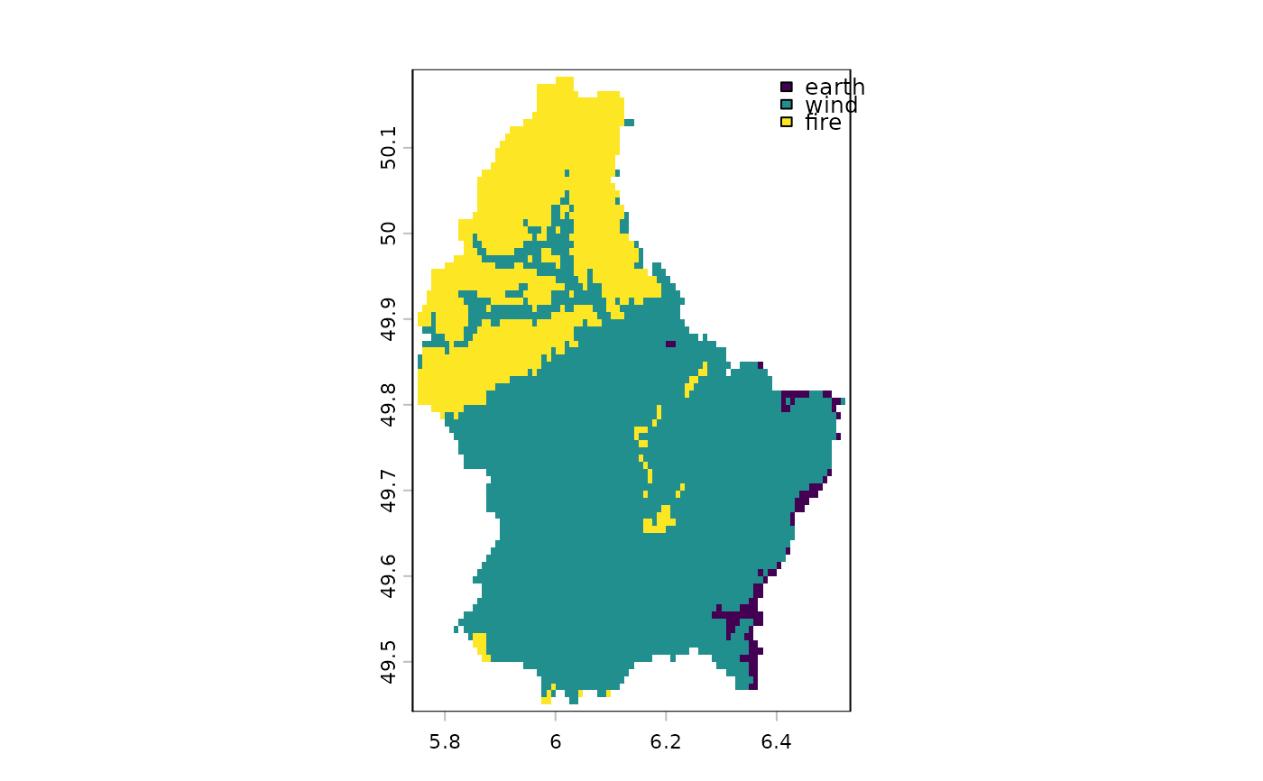
x <- trunc(r/200)
levels(x) <- data.frame(id=0:2, element=c("earth", "wind", "fire"))
plot(x, plg=list(x="topright"),mar=c(2,2,2,2))


oldpar <- par(no.readonly=TRUE)

# two plots with the same legend
dev.new(width=6, height=4, noRStudioGD = TRUE)
par(mfrow=c(1,2))
plot(r, range=c(50,600), mar=c(1,1,1,4))
plot(r/2, range=c(50,600), mar=c(1,1,1,4))

# as we only need one legend (also see the "panel" method):  
par(mfrow=c(1,2))
plot(r, range=c(50,600), mar=c(2, 2, 2, 2), plg=list(size=0.9, cex=.8), 
  pax=list(side=1:2, cex.axis=.6), box=FALSE)
#text(182500, 335000, "Two maps, one plot", xpd=NA)
plot(r/2, range=c(50,600), mar=c(2, 2, 2, 2), legend=FALSE, 
  pax=list(side=c(1,4), cex.axis=.6), box=FALSE)

par(oldpar)

# multi-layer with RGB
s <- rast(system.file("ex/logo.tif", package="terra"))   
s
#> class       : SpatRaster 
#> size        : 77, 101, 3  (nrow, ncol, nlyr)
#> resolution  : 1, 1  (x, y)
#> extent      : 0, 101, 0, 77  (xmin, xmax, ymin, ymax)
#> coord. ref. : Cartesian (Meter) 
#> source      : logo.tif 
#> colors RGB  : 1, 2, 3 
#> names       : red, green, blue 
#> min values  :   0,     0,    0 
#> max values  : 255,   255,  255 
plot(s)
# remove RGB
plot(s*1)
# or use layers
plot(s, 1)
plot(s, 1:3)

# fix legend by linking values and colors

x = rast(nrows = 2, ncols = 2, vals=1)
y = rast(nrows = 2, ncols = 2, vals=c(1,2,2,1))
cols = data.frame(id=1:2, col=c("red", "blue"))
plot(c(x,y), col=cols)

r  = rast(nrows=10, ncols=10, vals=1:100)
dr = data.frame(from=c(5,33,66,150), to=c(33, 66, 95,200), col=rainbow(4))
plot(r, col=dr)

### SpatVector 

f <- system.file("ex/lux.shp", package="terra")
v <- vect(f)

plot(v)

plot(v, "NAME_2", col=rainbow(12), border=c("gray", "blue"), lwd=3)

plot(v, 2, pax=list(side=1:2), plg=list(x=6.16, y=50.17, cex=.8), xlim=c(5.7, 6.7))

plot(v, 4, pax=list(side=1:2), plg=list(x=6.2, y=50.2, ncol=2), main="", box=FALSE)
 
plot(v, 1, plg=list(x=5.8, y=49.37, horiz=TRUE, cex=1.1), main="", mar=c(5,2,0.5,0.5))

plot(v, density=1:12, angle=seq(18, 360, 20), col=rainbow(12))


plot(v, "AREA", type="interval", breaks=3, mar=c(3.1, 3.1, 2.1, 3.1),
  plg=list(x="topright"), main="")

plot(v, "AREA", type="interval", breaks=c(0,200,250,350), 
  mar=c(2,2,2,2), xlim=c(5.7, 6.75),
  plg=list(legend=c("<200", "200-250", ">250"), cex=1, bty="o", 
  x=6.3, y=50.15, box.lwd=2, bg="light yellow", title="My legend"))

Usage

Arguments

See also

Examples